Speeding up Matlab plotting
This post describes my efforts at reducing the time it takes Matlab to render a time-series line plot, ultimately speeding up Matlab plotting in some cases by over 100x. Besides using OpenMP and SIMD in C-mex, I also got to learn a little bit about RAM bandwidth.
Code for this post can be found at: https://github.com/JimHokanson/plotBig_Matlab
Introduction
Normally plotting in Matlab is relatively uneventful. Plots render at reasonable rates and interacting with those plots is pleasant. Occasionally however, for large data sets, plotting seems to take forever.
This is particularly true for the type of data I work with that at times contains many tens, if not hundreds of millions of data points. Events lasting a couple hundred microseconds will be collected on scales of 10s of minutes to hours.
In reality plotting may take upwards of 10s of seconds (not forever). Zooming and panning then takes multiple seconds as well. This is not a long time for running a complicated batch analysis, but in the world of data exploration and analysis, in the world of user interaction, it is forever.
Ideally, this is something that Matlab would do better without requiring external tooling. In the mean time, I took to the internet to see if there was some way of plotting large data, specifically time-series line plots, more quickly in Matlab (more on what a time-series line plot is in a second).
I stumbled upon the following submission by Tucker McClure on the Mathworks File Exchange, https://www.mathworks.com/matlabcentral/fileexchange/40790-plot–big-. The code can also be found on GitHub at https://github.com/tuckermcclure/matlab-plot-big.
Although Tucker’s code noticeably sped up plotting, plots were still not plotting/updating as fast as I wanted. The following post describes my steps towards speeding up Matlab time-series plots even further, in some cases speeding up Matlab plotting by a factor of over 100x.
How to speed up plotting - plot less
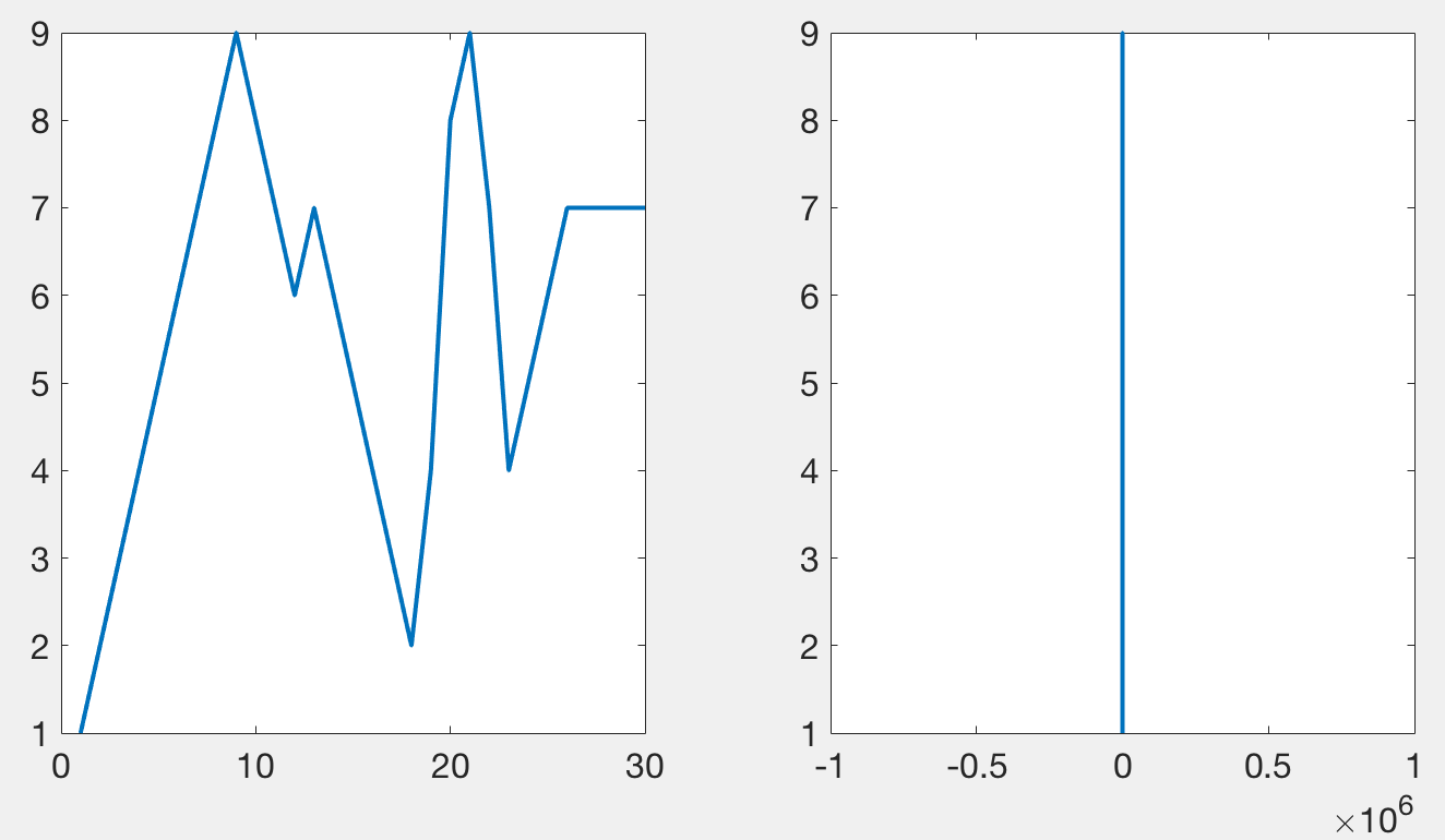
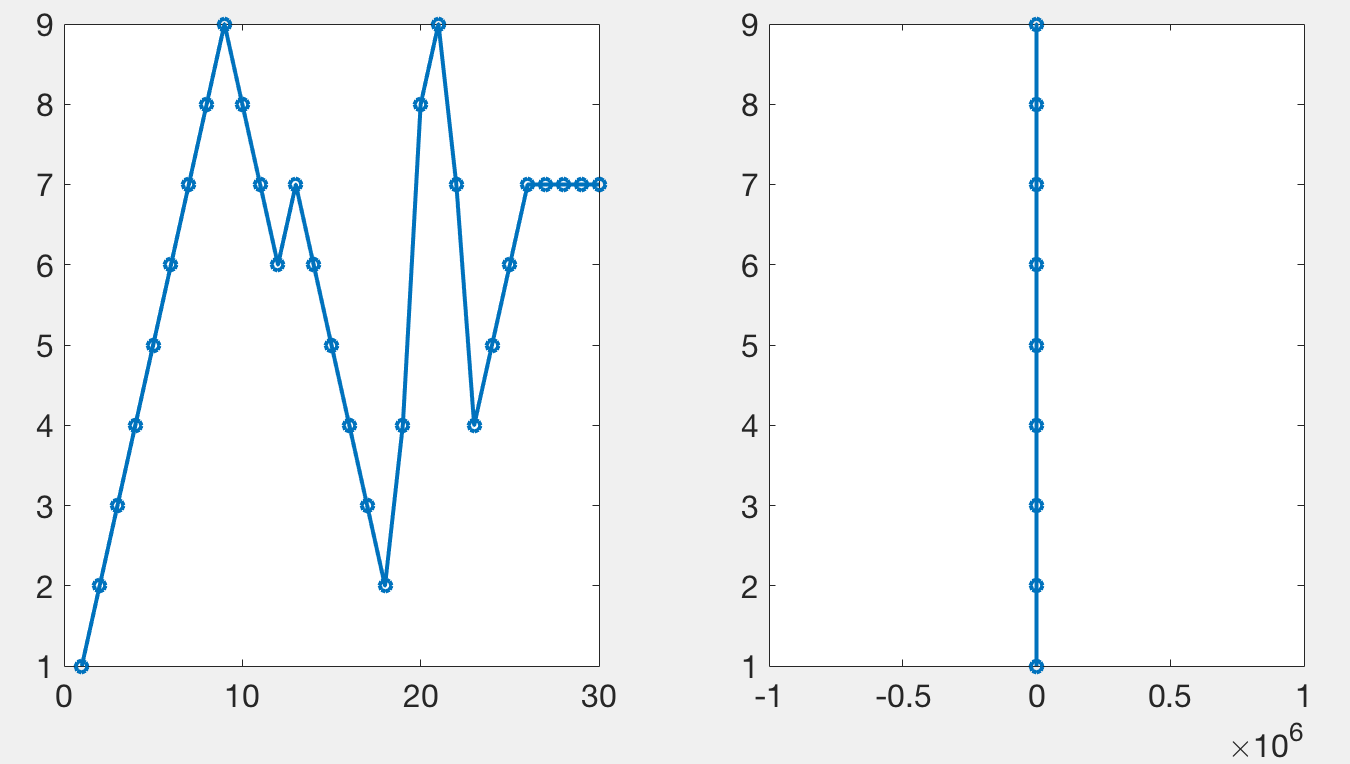
Tucker’s code, and mine, works by plotting only a subset of the data points in such a way that it looks like all of the data has been plotted. When plotting a lot of points, using lines, only the local maxima and minima are visible. The following figure demonstrates a simple signal (left) that when zoomed out appears as a vertical line (right) stretching from its maxima to its minima. This diagram is meant to illustrate that something which may look complex can be summarized by its extremes when only plotted over the width of a single pixel. Plotting anything besides the maxima and the minima does not add to any visual information, but can slow down the rendering of the graphic.
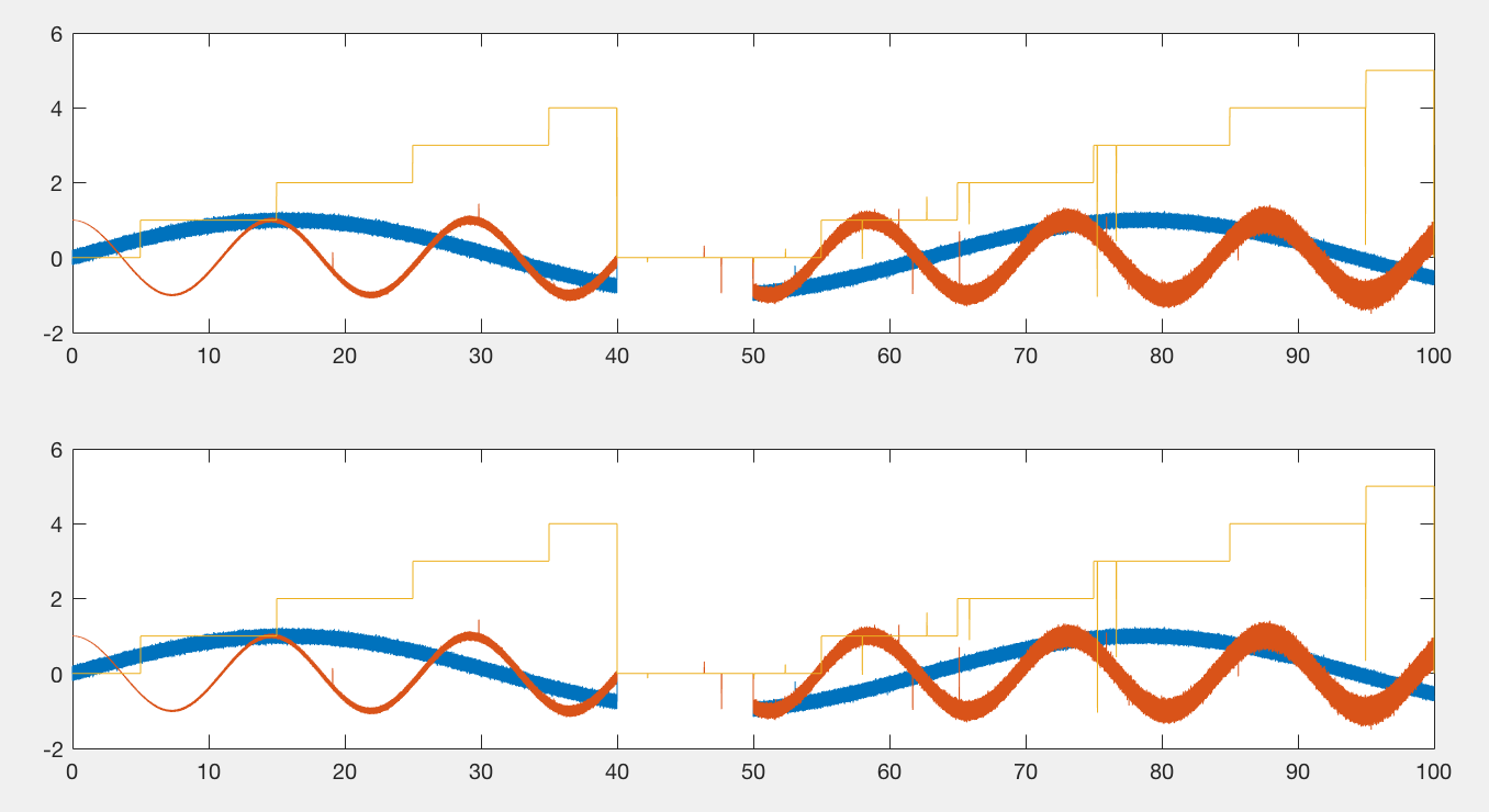
When done correctly, it should be impossible to tell the difference between the original plot and one that has been subsampled. The following figure has two axes. The first one contains 10000 points per line (3 lines total), the second one, 50 million. Rendering the first axes, using this code, takes about a second to render on my laptop. Rendering the second axes takes about 10 seconds. Importantly, they should appear the same.
So to reiterate, this code works by only plotting the maxima and minima on roughly a per pixel basis. Importantly, this is not a simple downsampling approach (e.g. take every 100th point), as this approach could miss extremes in the data.
Since only a subset of the data are plotted, callback routines need to be engaged in case the user zooms in to see more detail. Every time the user zooms a new subsample needs to be computed to again give the illusion that all the data has been plotted.
Plotting a time-series line plot
Based on the understanding that the data are subsampled so as to provide the illusion of plotting the entire data set, it is now possible to clarify in a more meaningful way the type of plot that this code covers.
This code requires:
- line plots
- time series data
By line plots, I mean plots where points are connected by lines, without markers. If markers were to be attached to a plot, the plot would no longer look the same by only plotting the extremes of the data.
By time series I mean a series of data points that are collected in time (increasing order). My code currently only handles evenly spaced data but it would be possible to expand to non-evenly spaced data. Critically though, the points that need to be considered for subsampling to a single pair of max and min points all need to be within the same chunk of time, rather than scattered throughout the array.
The impetus for improving upon the current solution
As mentioned earlier, the first solution that I tried was to use matlab-plot-big by Tucker McClure. Tucker’s code required a bit of information that I had not planned on providing to the plotting function, an array of timepoints (“x” data) associated with the “y” data.
Passing in an array of x-data points required doubling my memory requirements, since each y-value needs an x-value. This can be troublesome for large arrays that are close to the memory limits of my computer. In general I’m very slowly working on a Matlab object for time series data that carries abstract time information, rather than an x-vector, along with the data. Methods of this class can average the data aligned to specified times (events) or grab a subset of the data based on some epoch. These methods benefit from having time integrated with the data, rather than carrying around a separate time array. Importantly, by abstracting time into t0 (start-time) and dt (time-between-samples or the inverse of the sampling-rate), I no longer need to carry around an array that doubles the amount of memory required to work with my data.
While working on adding this feature to Tucker’s code, I couldn’t help but change a thing or two here and there. Eventually I decided to rewrite my own version from scratch.
Optimizations
The following outlines the optimizations I used to make this code fast. To make plotting fast I needed to make the data thinning routine fast. Thus, going forward, when talking about making the code fast, I am mostly referring to how to best compute min and max values over a subset of data such that this data, when plotted, looks like the original data.
These optimizations are presented in roughly chronological order of creation.
Finally, a bit of a disclaimer, I have zero formal training in writing C code (although technically I took a C++ class in high school, AP Computer Science!). I may have made some mistakes with the code, although my correctness tests (of which I admittedly need more) are passing and my performance tests are positive as well. That being said, there may be some room for improvement!
Constant Time
Tucker’s code supports non-evenly sampled data, which was not part of my use case. Thus one of the first things I did was to only support evenly sampled data.
To support non-evenly sampled data Tucker needs to find the start and stop time samples which correspond to the boundary of each pixel. Since I only work with evenly sampled data, I can use a simple formula to convert from a given time to sample. This formula is:
%t0 - start of time vector
%t - desired start or stop of data grabbing
%fs - sampling rate
sample = round((t - t0)*fs)+1;
Additionally, with sufficiently high oversampling, the groupings of chunks of data, from which I extract a single min and max are not important. In other words, if I wanted to grab roughly 100.5 samples per chunk, it doesn’t matter if I place the 101st sample in the first or second chunk. Even more generically, the samples per chunk is approximate, so I can change the 100.5 value to be 101 rather than trying to maintain 100.5 samples per chunk by toggling between 100 and 101 samples every other chunk.
So what does this all mean? It means that the execution loop never inspects any “x” data or never tries to adjust for some non-integer samples per chunk value. Instead we simply iterate over the data with fixed step sizes and grab the minimum and maximum of each chunk (subset) of data.
end_I = start_sample-1;
n = ... %calculate based on end_sample and samples_per_chunk
output_I = 0;
for i = 1:(n-1) %last chunk may be incomplete, so handle at the end
   start_I = end_I + 1;
   end_I = start_I + samples_per_chunk-1;
   output(output_I+1) = min(data(start_I:end_I));
   output(output_I+1) = max(data(start_I:end_I));
   output_I = output_I + 2;
end
//handle last chunk with similar code
If you look at the code you’ll also notice that I don’t keep track of whether the min or the max comes first. For vertical lines it doesn’t matter. This saves us needing to keep track track of the max and min indices, which saves on a lot of extra bookeeping and also enables some nice SIMD optimizations (see SIMD section). Note, this is not true for non-evenly sampled data. In that case you need to do a bit of extra work since large gaps between time points will expose the true order of the data. For evenly sampled data either the points are too dense to show these transitions or the length of the data to plot is too small (which would expose out of order subsampling) and thus the original data are plotted.
OpenMP
After some hacks in Matlab as well as getting some help from Jan Simon with getting a Matlab/C hybrid approach, I decided to write the entire subsampling code in C.
Matlab’s min() and max() functions are optimized to be multi-threaded. Matlab computes min and max values by splitting up portions of the array across multiple threads. As a simple example, computing the maximum value over 1 million data points can be accomplished by having two workers compute the maximum values over half of the data, then taking the maximum of the resulting two values (one max from each worker). This example could of course be expanded to even more workers (e.g. 4 workers taking 25% of the data).
Splitting the data up in this way however only makes sense if the number of samples to process is relatively large, since starting multiple threads has some overhead. Thus Matlab presumably does not implement a multi-threaded max until a specific number of samples are provided as an input.
Fortunately an even easier parallelization is possible for this task. Rather than splitting up calculation of the min and max values over a single data subset, it makes more sense to split up the subsets themselves. In other words, if we calculate the min and max values over 1000 chunks (subsets) of data, each 10000 points long, we will have each of our threads process a subset of the 1000 chunks, rather than each thread processing a portion of the 10000 points in each chunk.
This is relatively easy to accomplish with something called OpenMP. OpenMP consists of compiler directives and a set of library functions that make it really easy to split tasks across multiple threads. In particular, it is straightforward to write for loops where individual loops run in parallel. Here the only tricky part was that we had the potential for mutiple channels, each of which would need processing over chunks/subsets of the data. Potential ways of splitting the processing up are:
- 1 thread per channel
- threads process all channels for one chunk before moving to the next chunk
- threads process all chunks for one channel before moving to the next channel
Option 1 is not optimal if we have more threads than channels, as threads will sit idle. The typical use case is likely a single channel, so that may involve a lot of threads not doing anything. Options #2 and #3 are the same for a single channel, but one is clearly better than the other for multiple channels. Since a matrix containing multiple channels stores each channel’s data together, it is best to avoid repeatedly switching channels (option #2). Thus option #3 is what I am using.
The code below is what is used to split processing across multiple threads:
//OpenMP approach #1 (currently used)
//------------------------------------------------
#pragma omp parallel for simd collapse(2)
for (mwSize iChan = 0; iChan < n_chans; iChan++){
   for (mwSize iChunk = 0; iChunk < n_chunks; iChunk++){
       type *current_input_data_point = p_input_data + n_samples_data*iChan + iChunk*samples_per_chunk;
       type *local_output_data = p_output_data + n_outputs_per_chan*iChan + 2*iChunk;
There are two things to note in the above code. First, I’ve added the keyword “collapse” with “2” as an input, specifying that the OpenMP library should parallelize the following two “for” loops together. Without collapsing we would only split threads across channels. Second, order of execution of the loops is not guaranteed so we can’t update an iterator between the first and second for loop. Thus, I need to be able to determine where I need to start processing for the input and where to assign the output, based on a single calculation from the loop iterators, rather than by incrementing a counter.
As I will show below, this code speeds up the processing nicely relative to standard C code. There is however another type of parallelization that we can also use to speed up our code that is discussed in the next section.
SIMD
OpenMP is a method of using multiple-threads to speed up processing. Within a thread there are certain functions (instructions) that the processor can use which can work on multiple data points at the same time. This way of doing parallel computation is known as SIMD or “Single Instruction Multiple Data.” For example, one instruction “vpmaxub”, or alternatively accessed in C as “_mm256_max_epu8” computes the maximum of 32 8-bit unsigned integers “at once.” More specifically, the computation has some and others have specific latencies and throughputs, and these values may differ depending on the processor. So in some cases a function doing 32 operations “at once” may not be 32x faster than the function that does 1 operation, but it may be 8x faster, or 16x, or perhaps even 24.5x (some random number between 1x and 32x) faster.
Two other important disclaimers are needed when running SIMD. First, I’ve seen numerous examples of forcing code to be processed only with SIMD instructions. I haven’t timed the code I’ve seen but in many cases it is possible to generate SLOWER code by using SIMD, rather than faster (I think this is most likely especially true with excessive shuffling of bytes within a register). Ultimately profiling in this case is important.
Second, not all processors support these instructions, and new instructions get added from time to time. One of the latest instruction sets to be added is called AVX-512. As the name suggests it uses registers which can hold 512 bits (or 64 bytes - not bits - of data!). Thus one could use AVX-512 to process 8 doubles at once. At this time (February 2018) AVX-512 is only available on special processing boards (i.e. Xeon Phi) or very new server-grade processors. The first consumer grade processor support is coming this year. However, even when these new processors are released you will only be able to use AVX-512 instructions on computers with those processors. Older instructions must be used for older processors. Consumer grade processors with the previous set of instructions (AVX2 - with 256 bit wide registers) were first released in 2013.
The following shows a code snippet utilizing SIMD instructions to compute the max and min:
//Processing a "double" within the channel and subset loop
//---------------------------------------------------------
if (SIMD_ENABLED && s.HW_AVX && s.OS_AVX && samples_per_chunk > 4){
    INIT_MAIN_LOOP(double)
        getMinMaxDouble_SIMD_256(STD_INPUT_CALL);
    END_MAIN_LOOP
}else{
    INIT_MAIN_LOOP(double)
        getMinMaxDouble_Standard(STD_INPUT_CALL);
    END_MAIN_LOOP
}
//The SIMD processing code
//--------------------------------------------
void getMinMaxDouble_SIMD_256(STD_INPUT_DEFINE(double)){
    GET_MIN_MAX_SIMD(double,,4,__m256d,_mm256_loadu_pd,_mm256_max_pd,_mm256_min_pd,_mm256_storeu_pd)
}
//The generic SIMD processing function
//-------------------------------------------------------
#define GET_MIN_MAX_SIMD(TYPE,CAST,N_SIMD,SIMD_TYPE,LOAD,MAX,MIN,STORE) \
    SIMD_TYPE next;                         \
    SIMD_TYPE max_result;                   \
    SIMD_TYPE min_result;                   \
    TYPE max_output[N_SIMD];                \
	TYPE min_output[N_SIMD];                \
    TYPE min;                               \
    TYPE max;                               \
                                            \
    max_result = LOAD(CAST current_input_data_point); \
    min_result = max_result;                \
                                            \
    for (mwSize j = N_SIMD; j < (samples_per_chunk/N_SIMD)*N_SIMD; j+=N_SIMD){ \
        next = LOAD(CAST (current_input_data_point+j)); \
        max_result = MAX(max_result, next);             \
        min_result = MIN(min_result, next);             \
    }                                       \
                                            \
    /*Extract max values and reduce ...*/   \
    STORE(CAST max_output, max_result);     \
    STORE(CAST min_output, min_result);     \
                                            \
    /* Collapsing from a vector down to 1 sample */ \
    max = max_output[0];                    \
    for (int i = 1; i < N_SIMD; i++){       \
        if (max_output[i] > max){           \
            max = max_output[i];            \
        }                                   \
    }                                       \
    min = min_output[0];                    \
    for (int i = 1; i < N_SIMD; i++){       \
        if (min_output[i] < min){           \
            min = min_output[i];            \
        }                                   \
    }                                       \
                                            \
    /* leftovers processing */ \
    for (mwSize j = (samples_per_chunk/N_SIMD)*N_SIMD; j < samples_per_chunk; j++){ \
        if (*(current_input_data_point + j) > max){             \
            max = *(current_input_data_point + j);              \
        }else if (*(current_input_data_point + j) < min){       \
            min = *(current_input_data_point + j);              \
        }                                                       \
    }                                                           \
                                                                \
    *min_out = min;                                             \
    *max_out = max;
//The standard loop
//-----------------------------------------------
#define GET_MIN_MAX_STANDARD(TYPE)              \
	TYPE min = *current_input_data_point;       \
 	TYPE max = *current_input_data_point;       \
                                                \
    for (mwSize iSample = 1; iSample < samples_per_chunk; iSample++){    \
        if (*(++current_input_data_point) > max){   \
            max = *current_input_data_point;        \
        }else if (*current_input_data_point < min){ \
            min = *current_input_data_point;        \
        }                                           \
    }                                               \
                                                    \
    *min_out = min;                                 \
    *max_out = max;
A summary of the code is as follows:
- Switch processing depending upon data type (double shown)
- Loop over channels and chunks (subsets of the channel data). (See OpenMP above)
- Within each subset process according to the supported SIMD type (See more details below).
- A final function at the end that processes the last subset that was not of the standard size. (Not discussed further).
The code above is the actual code that I’m currently using and it contains a lot of macros to support different data types. Below I’ve rewritten a portion of the actual SIMD code for doubles.
    __m256d next;
    __m256d max_result;
    __m256d min_result;
    double max_output[4];
	  double min_output[4];
    double min;
    double max;

    //The first "n" values (in this case 4) start as our
    //min and max data points
    max_result = _mm256_loadu_pd(current_input_data_point);
    min_result = max_result;

    //Load the next "n" data points and compute the min and
    //max of our current leaders (min_result,max_result) vs
    //the current array. Do this over all the data
    //that we can that evenly divides by the register size.
    //Since we are using double (8 bytes) with 32 byte registers
    //we process in sets of 4 (32/8)
    for (mwSize j = 4; j < (samples_per_chunk/4)*4; j+=4){
        next = _mm256_loadu_pd(current_input_data_point+j);
        max_result = _mm256_max_pd(max_result, next);
        min_result = _mm256_min_pd(min_result, next);
    }

    //Transfer our results from the registers
    //back into normal data types
    _mm256_storeu_pd(max_output, max_result);
    _mm256_storeu_pd(min_output, min_result);

    //The current values for max_output and min_output
    //have "n" total values, one of which is the actual
    //max and min. The others are only the max and min
    //for every "nth" value.
    //
    //For example, for doubles, the
    //first entry is the max value for the 1st, 5th, 9th, 13th
    //etc values in the original array. The second entry
    //is the max value for the 2nd, 6th, 10th, 14th, etc. values
    //in the original array.

    //Collapsing to a single max
    max = max_output[0];
    for (int i = 1; i < 4; i++){
        if (max_output[i] > max){
            max = max_output[i];
        }
    }

    //Collapsing to a single min
    min = min_output[0];
    for (int i = 1; i < 4; i++){
        if (min_output[i] < min){
            min = min_output[i];
        }
    }

    //Leftover processing
    for (mwSize j = (samples_per_chunk/4)*4; j < samples_per_chunk; j++){
        if (*(current_input_data_point + j) > max){
            max = *(current_input_data_point + j);
        }else if (*(current_input_data_point + j) < min){
            min = *(current_input_data_point + j);
        }
    }

    *min_out = min;
    *max_out = max;
I’ve tried to comment the code above to clarify how this code works. There is however one aspect of this processing that was not immediately obvious to me, and that should be explained explicitly. In general SIMD instructions are designed to work on independent arrays, rather than on subsets of an original array. For example with addition, the standard example is:
//Ammenable to SIMD
//------------------------------
c[0] = a[0] + b[0];
c[1] = a[1] + b[1];
c[2] = a[2] + b[2];
However, if we want to add all elements together, we might try and get SIMD to do something like:
//Not good for SIMD
//----------------------------
c = a[0] + a[1] + a[2] + a[3]
This approach in general is not good for SIMD, as there are few, if any, instructions that collapse multiple elements of an array into a single value in this way. However, what I’ve found to work quite well is to keep an intermediate temporary variable that I continually evaluate against different parts of the array. So for addition something like this:
//Approach to summing all elements of "a"
//--------------------------------------
//Initialize
c[0] = a[0];
c[1] = a[1];

//This would typically be done in a loop ...
//The addition (or other operation) would be
//done with SIMD calls

//Loop iteration 0
//------------------------------
//Add next n elements (using SIMD)
//These n statements would be done in parallel
//because of the SIMD call
c[0] = c[0] + a[2];
c[1] = c[1] + a[3];

//Loop iteration 1
//------------------------------
//Add next n elements in parallel (using SIMD)
c[0] = c[0] + a[4];
c[1] = c[1] + a[5];

//Loop iteration 2
//------------------------------
//Add next n elements in parallel (using SIMD)
c[0] = c[0] + a[6];
c[1] = c[1] + a[7];

//etc.

//Finally, collapse output (not using SIMD)
output = c[0] + c[1];
For simplicity the above example uses only 2 new array elements at a time, when in reality the minimum in the code is 4 (doubles) and up to 32 values at a time for uint8 and int8 data types.
In general it is good to allow multiple statements to execute independently, rather than having each statement depend on the next one. For example in the previous example, each iteration depended on the previous loop because of the ‘c’ elements. If we remove, or even just lessen the dependencies in the loop, this allows us to execute a third type of parallelism (besides across threads and SIMD), called superscaler processing. Essentially modern processors are capable of executing the same instruction multiple times on the same thread if there are no dependencies.
For example, ignoring SIMD for a second, the following two instructions could execute at the same time since there are no dependencies:
//May execute simultaneously, even without SIMD
//I think ...
//---------------------------------------------
c[0] = a[0] + a[1];
c[1] = a[2] + a[3];
However, if we add a dependency, like in the example below, we can’t execute both instructions in the same clock cycle:
//Can't execute simultaneously, due to dependencies
//----------------------------------------------------
c[0] = a[0] + a[1];
c[1] = c[0] + a[2]; //requires output from first statement
So for SIMD, we might get better behavior if our loop had two seperate (or more) temporary variables, rather than just one. If we had two temporary variables, this would halve the number of required loops, since each temporary variable is operating on half of the data.
//Approach to summing all elements of "a"
//--------------------------------------
//Now trying to take advantage of superscalar processing
//Initialize
c[0] = a[0];
c[1] = a[1];
d[0] = a[2]; //Notice this is a different output than "c"
d[1] = a[3];

//Loop iteration 0
//--------------------------------------------
//These 2 execute simultaneously using SIMD
c[0] = c[0] + a[4];
c[1] = c[1] + a[5];

//These 2 executed simultaneously using SIMD
d[0] = d[0] + a[6];
d[1] = d[1] + a[7];

//** Because of superscalar processing, we might be able to
//execute the adding of the "c" and "d" vectors at the same time.


//Loop iteration 1
//--------------------------------------------
//These 2 execute simultaneously using SIMD
c[0] = c[0] + a[8];
c[1] = c[1] + a[9];

//These 2 executed simultaneously using SIMD
d[0] = d[0] + a[10];
d[1] = d[1] + a[11];

//** Again, because of superscalar processing
//"c" and "d" may get evaluated at the same time

//etc.

//Finally, collapse output (not using SIMD)
output = c[0] + c[1] + d[0] + d[1];
In some initial testing, I could get speedups by writing code to take advantage of superscalar processing (and possibly pipelining, a related technique that CPUs use). Fortunately, once I remembered to enable compiler optimizations, these differences went away. In other words, the compiler seems to be able to do a good enough job rewriting my loops to optimize these parallelization techniques.
Regarding compilers: online I’ve seen many statements to the effect that a compiler will be able to fix code to make it as fast as possible. My general experience however has been that compilers are not very good at generating parallel code. However, in this case, the compiler (gcc) appears to do a pretty good job of optimizing this aspect of my code (superscalar processing and pipelining).
So to summarize the SIMD section:
SIMD instructions can speed up execution of basic functions like adding or computing a maximum of elements by working on multiple elements at once, rather than one element at a time. By continually evaluating subsets of an array against a temporary variable, we are able to reduce an array from its original size down to one that is the same length as the SIMD registers. This array is then collapsed further into a single value - the answer, such as the maximum or minimum of an array - using standard C. In theory we can do better than a “for” loop when each iteration is independent (superscalar processing). Fortunately however the compiler seems to take care of this aspect of the code for us, but only if optimizations are enabled!
Data Reduction Results
The following graphs demonstrate the speedup seen by using various optimization approaches on three different computers relative to the same code in Matlab.
These computers are:
| Name | CPU | cores | Memory | OS | SIMD |
|---|---|---|---|---|---|
| Turtle | i5-3570 @ 3.4GHz | 2 | Dual Chan DDR3 1333 | Win 7 | AVX |
| Paladin | i7-4770 @ 3.4GHz | 4 | Dual Chan DDR3 1333 | Win 10 | AVX2 |
| Jim’s Macbook | m3-6Y30 @ 1.1GHz | 2 | Dual Chan DDR3 1866 | Mac OS | AVX2 |
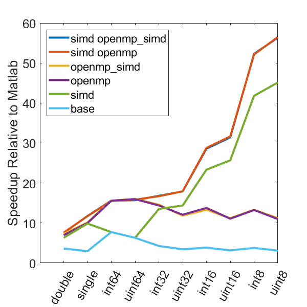
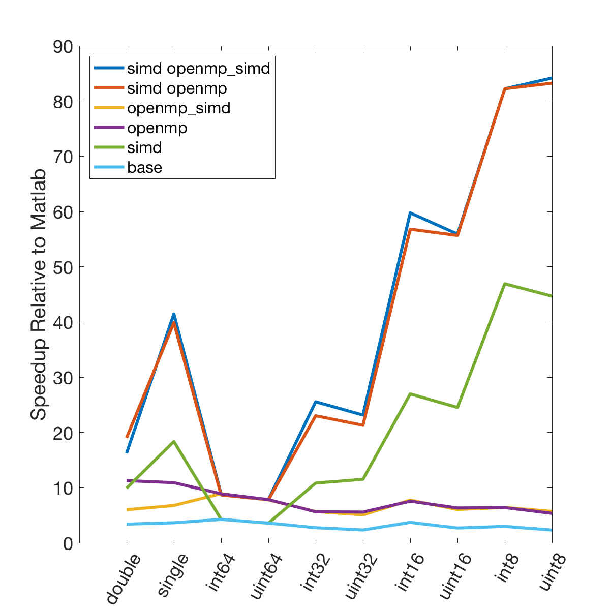
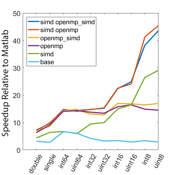
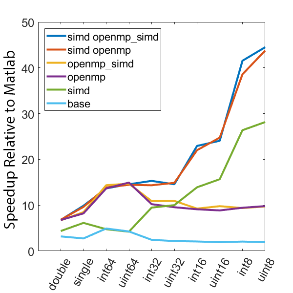
The following test computes min and max values every 5000 samples over 50 million data points. All execution times are normalized to the time it takes to execute the computation using only the Matlab language. Different data types are tested, as well as different compilation configurations. These configurations are as follows, all compiled with the “-O3” optimization level:
- base - regular C code, no OpenMP or SIMD
- simd - SIMD only, no OpenMP
- openmp - OpenMP only, no SIMD
- openmp_simd - OpenMP with SIMD flag (see below)
- simd openmp - OpenMP and SIMD
- simd openmp_simd - OpenMP with SIMD flag, and SIMD
The SIMD flag for OpenMP (openmp_simd, “#pragma omp parallel for simd”) was a bit confusing. My current understanding is that it is a hint to the compiler to try and use SIMD in the OpenMP code. Importantly, based on the speed results it is pretty clear that the SIMD flag is not required to enable the use of SIMD instructions in the code.
One final note before the results. These results were all compiled using GCC. For my Mac this involved downloading GCC via Homebrew (v6.2?). For Windows I initially used TDM-GCC, which currently supports GCC 5.1. For this project I also downloaded mingw64. Use of GCC was an important part of a previous project, and most likely wasn’t necessary for this one, but it was what I had setup.
Onto the results:
| A: Turtle mingw64 | B: Mac gcc |
|---|---|
|
|
| C: Paladin mingw64 | D: Paladin tdm-gcc |
|
|
There is a lot of information in these figure panels. Some things of note are:
-
SIMD shows a large speedup as a function of the data size. 8-bit numbers are processed up to ~85x faster (mac) with SIMD and OPENMP compared to base Matlab. I generally don’t plot 8-bit numbers, but fast 16-bit numbers could be useful since DAQ data is typically collected as 16 bit numbers. The general idea is that you would compute max and min values based on the 16-bit data, and then scale dynamically afterwards when rendering.
-
Base C is not that much faster than Matlab. I don’t have the exact numbers in front of me but from the graphs it is roughly 3 - 4x faster to use C than Matlab (as opposed to 10 - 100x). Matlab has made significant speedups throughout the years and I rarely bother anymore to try and vectorize code that isn’t easily vectorizable, I just write for loops.
-
OpenMP with the SIMD flag (openmp_simd) doesn’t do much if anything compared to just OpenMP. If it did that would be great, but this says that compilers aren’t to the point yet where they can magically insert SIMD code everywhere and make everything faster.
-
SIMD code with OpenMP doesn’t scale as much as I expected. I’ve read that the expected speedup can be multiplicative, but that doesn’t appear to be the case for this code. My guess is most likely I’ve hit memory bandwidth limitations. I will address this in the next section when we look at execution time.
-
The speedup on my mac for doubles and singles is surprising. The reason for this is unclear.
-
mingw64 is a bit faster than tdm-gcc for some of the 8, 16, and 32 bit values. Since these are both using gcc I take this as an indication of the speed improvement that occurs over time. The best option however (simd openmp) is comparable across all data types.
Speed Comparison
The previous results examined how quickly I could compute data values to plot. They however did not indicate how quickly plotting occurred. Initial testing was done for a variety of plot sizes and data types for Matlab, Tucker’s code, and my code. In testing Tucker’s code was surprisingly about the same speed as standard Matlab code. Further testing revealed that the relative speed depended on which version of Matlab I was using.
The following plot shows the time it takes to plot 100 million point of data type “double” for different Matlab versions on my Turtle computer.

The figure shows relatively consistent behavior across different Matlab versions for my code and Tucker’s code. With different versions the default Matlab plotting performance has changed. In particular there has been a noticeable improvement with newer versions. The peak at 2014b is from the transition to a new graphics system, HG2 and I’m not entirely sure why there was a dip with 2016b that didn’t persist in the 2017 versions. Based on this test, Tucker’s code looks to be currently irrelevant. However, this test was only for one channel. Based on how Tucker’s code works, I would expect faster performance relative to Matlab for plotting multiple channels - in the same matrix input - since he only has to pay a time computation penalty once. Additionally, these times are only for initial plots, not for plot manipulations (zooming, panning). Again, I would expect Tucker’s code to show improvements relative to Matlab in these areas.
The average execution time for my code was 61 ms. In 2017b the time for the C-mex code to generate min/max values from the 100 million data points was 42 ms. Thus generating the subsampled data still takes a relatively large portion (69%) of the total plot time. However, even though further speed improvements are possible, plotting now takes a reasonable amount of time, which was my main goal for this endeavor.
Finally, I’ll mention relative speedups, even though I think the absolute speed is a bit more important here. For 2017b on Turtle the speedup for the 100 million data points was 74x. For 100 milion data points of “single” data type, the speedup was 106. At 300 million data points these values were 79x and 112x respectively.
A brief memory aside
Processing 100 million samples of type double requires loading 0.8 GB of data. I’m not exactly sure of the memory sticks that are in Turtle but I’m operating at approximately 667 MHz according to a program called CPU-Z. Somewhere I read that memory actually gets transferred on both rising and falling edges of the clock, so the speed is actually twice the clock rate (so roughly 1333 MHz). Thus my memory is labeled as DDR3 1333 MHz. The DDR3 is something else CPU-Z told me, it isn’t calculated, although there is generally correspondence between speeds and DDR type so it could be inferred. These chips transfer 64 bits at a time, so the data transfer rate is 1333*64 bits or 85312 Mb/s (Mb due to the clock speed being in MHz) or 10664 MB/s or 10.6 GB/s. Note that in addition to seeing DDR-1333 it is also common to see something like PC3-10600 which corresponds to the MB/s value.
When reading about these numbers most websites cautioned that these are maximum values and that due to unspecified factors getting this througput for a sustained period of time can be difficult. Assuming the processor and the cache are working together in a smart way it is not clear to me what exactly these factors are.
The actual memory throughput, in GB/s also depends on another factor, called the memory channel architecture. Dual-channel memory, which is now relatively common, doubles the bandwidth if multiple RAM slots are populated. This would bring the expected max throughput to 21.2 GB/s. For reference Quad-channel memory also exists (for a 4x throughput), but its not nearly as common. Note that even though my 2014 computer (Paladin) has 4 RAM slots, it is still only operating in dual-channel mode (due to the motherboard and processor). So it is incorrect to multiply the number of RAM slots by single-channel memory throughput to get total memory throughput.
If we calculate how long it would take to load all data from RAM into the processor I arrive at 38 ms (0.8 GB of data / 21.2 GB/s). My execution time has a bit of overhead besides just loading the data into the processor to compute min and max values. Even if we ignore the overhead, our throughput is about 90% of the maximum (and most likely even higher). From online reading it seems like something in that range is pretty darn good.
Importantly, these numbers suggest that the subsampling routine is almost certainly memory limited. This explains why we don’t see drastic speed ups from the use of OpenMP and multiple cores (Figure 5). This may also explain why my mac, which has faster memory, benefits more from combining SIMD and OpenMP.
Summary
By using OpenMP and SIMD in C-mex code I was able to generate fast code for subsampling data. In particular I was pretty excited about figuring out how to use SIMD to operate across variables within an array, since I had not seen this disucssed before online. Realizing that the order of max and min data points doesn’t matter simplified the code significantly and led to a large speedup as well. These plotting routines are now my goto functions for plotting time-series line data because I don’t have to wait for plots to render, minimizing distractions and improving data exploration.
The transition out of a hybrid Matlab/C approach was motivated by the desire to be able to scroll (pan) fast, specifically for plotting data during data collection. The changes discussed in this post have helped to improve scrolling tremendously. There were however a few improvements and additions that were scrolling specific which I hope to cover in a later post.